Code
library(tidyverse)
library(tidymodels)
library(factoextra)

income_data <- read_csv("../data/adult_income_dataset.csv")Using tidymodels
This document demonstrates how to perform clustering in R using the tidymodels framework. Clustering is an unsupervised learning technique that groups similar data points together based on their inherent characteristics. We will use the adult_income_dataset.csv for this demonstration.
First, we load the necessary libraries and the income dataset.
library(tidyverse)
library(tidymodels)
library(factoextra)
income_data <- read_csv("../data/adult_income_dataset.csv")glimpse(income_data)Rows: 32,561
Columns: 15
$ age <dbl> 39, 50, 38, 53, 28, 37, 49, 52, 31, 42, 37, 30, 23, 3…
$ workclass <chr> "State-gov", "Self-emp-not-inc", "Private", "Private"…
$ fnlwgt <dbl> 77516, 83311, 215646, 234721, 338409, 284582, 160187,…
$ education <chr> "Bachelors", "Bachelors", "HS-grad", "11th", "Bachelo…
$ `education-num` <dbl> 13, 13, 9, 7, 13, 14, 5, 9, 14, 13, 10, 13, 13, 12, 1…
$ `marital-status` <chr> "Never-married", "Married-civ-spouse", "Divorced", "M…
$ occupation <chr> "Adm-clerical", "Exec-managerial", "Handlers-cleaners…
$ relationship <chr> "Not-in-family", "Husband", "Not-in-family", "Husband…
$ race <chr> "White", "White", "White", "Black", "Black", "White",…
$ sex <chr> "Male", "Male", "Male", "Male", "Female", "Female", "…
$ `capital-gain` <dbl> 2174, 0, 0, 0, 0, 0, 0, 0, 14084, 5178, 0, 0, 0, 0, 0…
$ `capital-loss` <dbl> 0, 0, 0, 0, 0, 0, 0, 0, 0, 0, 0, 0, 0, 0, 0, 0, 0, 0,…
$ `hours-per-week` <dbl> 40, 13, 40, 40, 40, 40, 16, 45, 50, 40, 80, 40, 30, 5…
$ `native-country` <chr> "United-States", "United-States", "United-States", "U…
$ income <chr> "<=50K", "<=50K", "<=50K", "<=50K", "<=50K", "<=50K",…income_data |> count(race)# A tibble: 5 × 2
race n
<chr> <int>
1 Amer-Indian-Eskimo 311
2 Asian-Pac-Islander 1039
3 Black 3124
4 Other 271
5 White 27816# For simplicity, we'll remove rows with any missing values
income_data_clean <- income_data %>%
select(-race) %>%
na.omit() %>%
sample_n(1000) # Randomly sample 10,000 rowsglimpse(income_data_clean)Rows: 1,000
Columns: 14
$ age <dbl> 19, 51, 57, 23, 47, 23, 40, 32, 37, 27, 26, 42, 40, 3…
$ workclass <chr> "Private", "Private", "State-gov", "Self-emp-inc", "P…
$ fnlwgt <dbl> 47577, 302847, 19520, 214542, 117849, 292023, 280362,…
$ education <chr> "Some-college", "HS-grad", "Doctorate", "Some-college…
$ `education-num` <dbl> 10, 9, 16, 10, 12, 9, 9, 14, 9, 9, 9, 12, 9, 9, 9, 10…
$ `marital-status` <chr> "Never-married", "Married-civ-spouse", "Divorced", "N…
$ occupation <chr> "Transport-moving", "Craft-repair", "Prof-specialty",…
$ relationship <chr> "Not-in-family", "Husband", "Unmarried", "Not-in-fami…
$ sex <chr> "Male", "Male", "Female", "Male", "Male", "Male", "Ma…
$ `capital-gain` <dbl> 0, 0, 0, 0, 0, 0, 0, 0, 0, 0, 0, 0, 0, 0, 0, 0, 0, 0,…
$ `capital-loss` <dbl> 0, 0, 0, 0, 0, 0, 0, 0, 0, 0, 0, 0, 0, 0, 0, 0, 0, 0,…
$ `hours-per-week` <dbl> 50, 54, 50, 50, 44, 45, 35, 40, 40, 40, 40, 40, 84, 6…
$ `native-country` <chr> "United-States", "United-States", "United-States", "U…
$ income <chr> "<=50K", "<=50K", "<=50K", "<=50K", "<=50K", "<=50K",…# Preprocessing using recipes
library(recipes)
income_recipe <- recipe(~ ., data = income_data_clean) %>%
step_dummy(all_nominal_predictors()) %>% # One-hot encode all nominal (categorical) predictors
step_normalize(all_numeric_predictors()) %>% # Normalize all numerical predictors
prep(training = income_data_clean)
income_data_processed <- bake(income_recipe, new_data = income_data_clean)
# Remove any columns that might have resulted in all zeros after one-hot encoding if they were constant
income_data_processed <- income_data_processed[, colSums(income_data_processed) != 0]The Elbow Method is a heuristic used to determine the optimal number of clusters in a dataset. We can visualize the total within-cluster sum of squares as a function of the number of clusters.
fviz_nbclust(income_data_processed, kmeans, method = "wss") +
  labs(subtitle = "Elbow Method")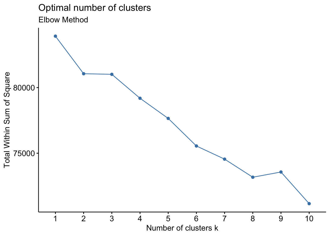
K-Means is a popular clustering algorithm. We will use it to group the income data into clusters. The optimal number of clusters can be determined from the Elbow Method plot.
set.seed(123)
kmeans_model <- kmeans(income_data_processed, centers = 5, nstart = 25) # Assuming 2 clusters from Elbow Method

# Visualize the clusters (using first two principal components for visualization)
fviz_cluster(kmeans_model, data = income_data_processed)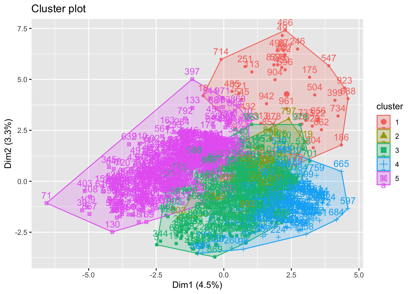
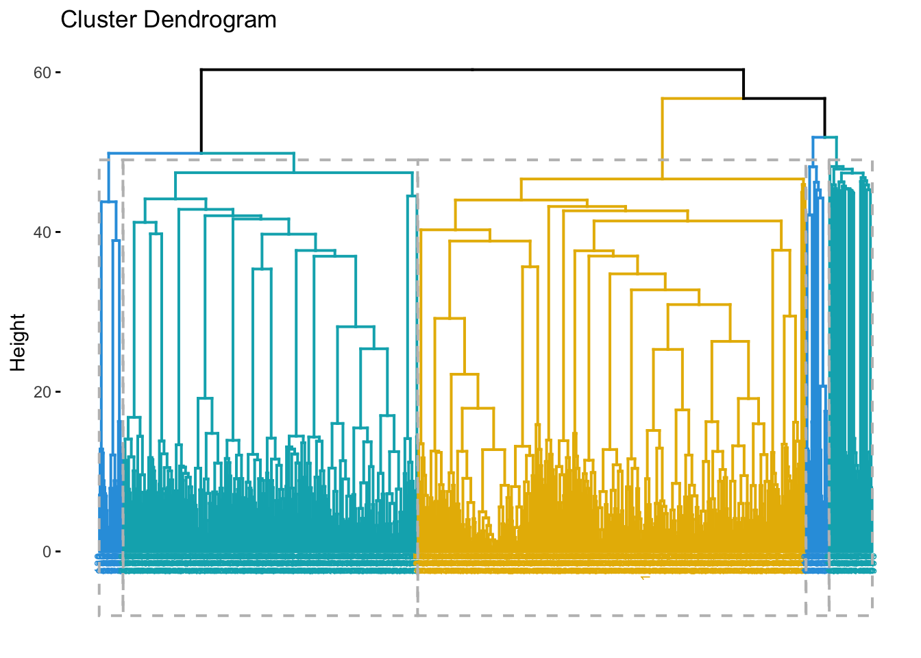
Hierarchical clustering is another common clustering method.
# Calculate the distance matrix
dist_matrix <- dist(income_data_processed, method = "euclidean")

# Perform hierarchical clustering
hclust_model <- hclust(dist_matrix, method = "ward.D2")

# Visualize the dendrogram
fviz_dend(hclust_model, k = 5,
          cex = 0.5, # label size
          k_colors = c("#2E9FDF", "#00AFBB", "#E7B800"),
          color_labels_by_k = TRUE, # color labels by groups
          rect = TRUE # Add rectangle around groups
          )
Here’s a comparison of K-Means and Hierarchical Clustering:
|:——————–|:————————————————-|:—————-:————————————-| | Approach | Partitioning (divides data into k clusters) | Agglomerative (bottom-up) or Divisive (top-down) | | Number of Clusters | Requires pre-specification (k) | Does not require pre-specification; dendrogram helps | | Computational Cost | Faster for large datasets | Slower for large datasets (O(n^3) or O(n^2)) | | Cluster Shape | Tends to form spherical clusters | Can discover arbitrarily shaped clusters | | Sensitivity to Outliers | Sensitive to outliers | Less sensitive to outliers | | Interpretability | Easy to interpret | Dendrogram can be complex for large datasets | | Reproducibility | Can vary with initial centroids (unless fixed) | Reproducible |
This document provided a brief overview of clustering in R using tidymodels. We demonstrated both K-Means and Hierarchical clustering on the income dataset.